Introduction
Besides the impulse response, denoted by $h[n]$, and the Difference Equation (DE) we will see that the frequency response is an alternative description of an FIR filter. Obviously all these different descriptions are related to each other and each of the descriptions has its own advantage. The advantage of the frequency response description is that we can fairly easily see the response of the FIR to frequencies.
Screencast video [⯈]
Module overview
This module covers the following topics:
- Frequency response - This section will introduce the frequency response and will derive the frequency response of an arbitrary FIR filter.
- Properties [⯈] - As will all other transforms, the frequency response has some properties which ease the calculations.
Exercises
In this section several exercises are available, including their answers. The exercises marked in blue are explained by means of more extensive pencast videos.
Video quiz
Exercise bundle
Answers
Download the answers here.
Pencast videos [⯈]
The above video player contains a playlist of all pencast videos which can be expanded by clicking the playlist icon in the upper-right corner.
MATLAB lab
Accompanied to this modules are some exercises in MATLAB, which will test your knowledge of the module and will help improve your MATLAB skills.
Lab assignment
MATLAB demo [⯈]
Summary
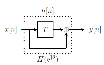
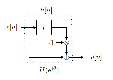
Relationship impulse response and frequency response: $$ \boxed{ \begin{eqnarray*} \text{Time domain} & \circ \hspace{-2.3mm} - \hspace{-1.1mm} \circ & \text{Frequency domain} \newline h[n]= \sum_{k=0}^{M-1} h[k] \delta[n-k] & \circ \hspace{-2.3mm} - \hspace{-1.1mm} \circ & H(e^{j{\theta}})= \sum_{k=0}^{M-1} h[k] e^{-j{\theta k}} \end{eqnarray*} } $$
Basic FIR property:
When applying a sum of frequencies $x[n] = A_0 + \sum_{k=1}^{N} A_k \cos ( \theta_k n + \phi_k)$ to an FIR filter with frequency response $H(e^{j{\theta}}) = |H(e^{j\theta})| e^{j{\angle{H(e^{j{\theta}})}}}$ then the output can be written as follows: $$ y[n] = |H(e^{j0})| + \sum_{k=1}^{N} |H(e^{j\theta_k})| A_k \cos (\theta_k n + \phi_k + \angle{H(e^{j\theta_k})}) $$
Properties frequency response $$ \boxed{ \begin{eqnarray*} \text{Periodic } & : & H(e^{j\theta}) = H(e^{j(\theta + l \cdot 2 \pi)}) \newline \text{Complex conjugated } & : & H(e^{-j\theta}) = (H(e^{j\theta}))^\ast \end{eqnarray*} } $$
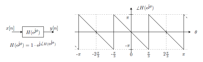
Graphical representation:
- Both Magnitude- and phase- response are depicted in the Fundamental Interval (FI): $|\theta| \leq \pi$.
- The phase response is depicted in the range $|\angle{H(e^{j\theta})}| \leq \pi$.
- A phase jump of $\pm \pi$ is applied in the phase response plot for each zero crossing of the magnitude response.
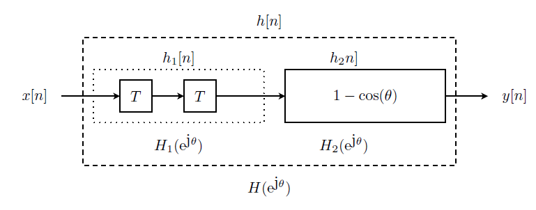
Cascading FIR filters:
Convolution in time- is equivalent to multiplication in frequency-domain: $$ \boxed{ h_1[n] * h_2[n] \hspace{3mm} \circ \hspace{-2.3mm} - \hspace{-1.1mm} \circ \hspace{3mm} H_1(e^{j\theta}) \cdot H_2(e^{j\theta}) } $$
Steady state and transient behaviour:
- Transient region: The complex multiplier $\left ( \sum_{k=0}^{{\color{red}{n}}} h[k] e^{-j\theta_1 k} \right )$ depends on the index $n$.
- Steady state region: The complex multiplier $\sum_{k=0}^{{\color{blue}{M-1}}} h[k] e^{-j\theta_1 k}$ is constant. Output contains only input frequency ($\theta_1$ in this example).
- If for $n > M-1$ the input changes to zero or to another frequency $\theta_2 \neq \theta_1$, then there will be a new transition- and steady state- region.